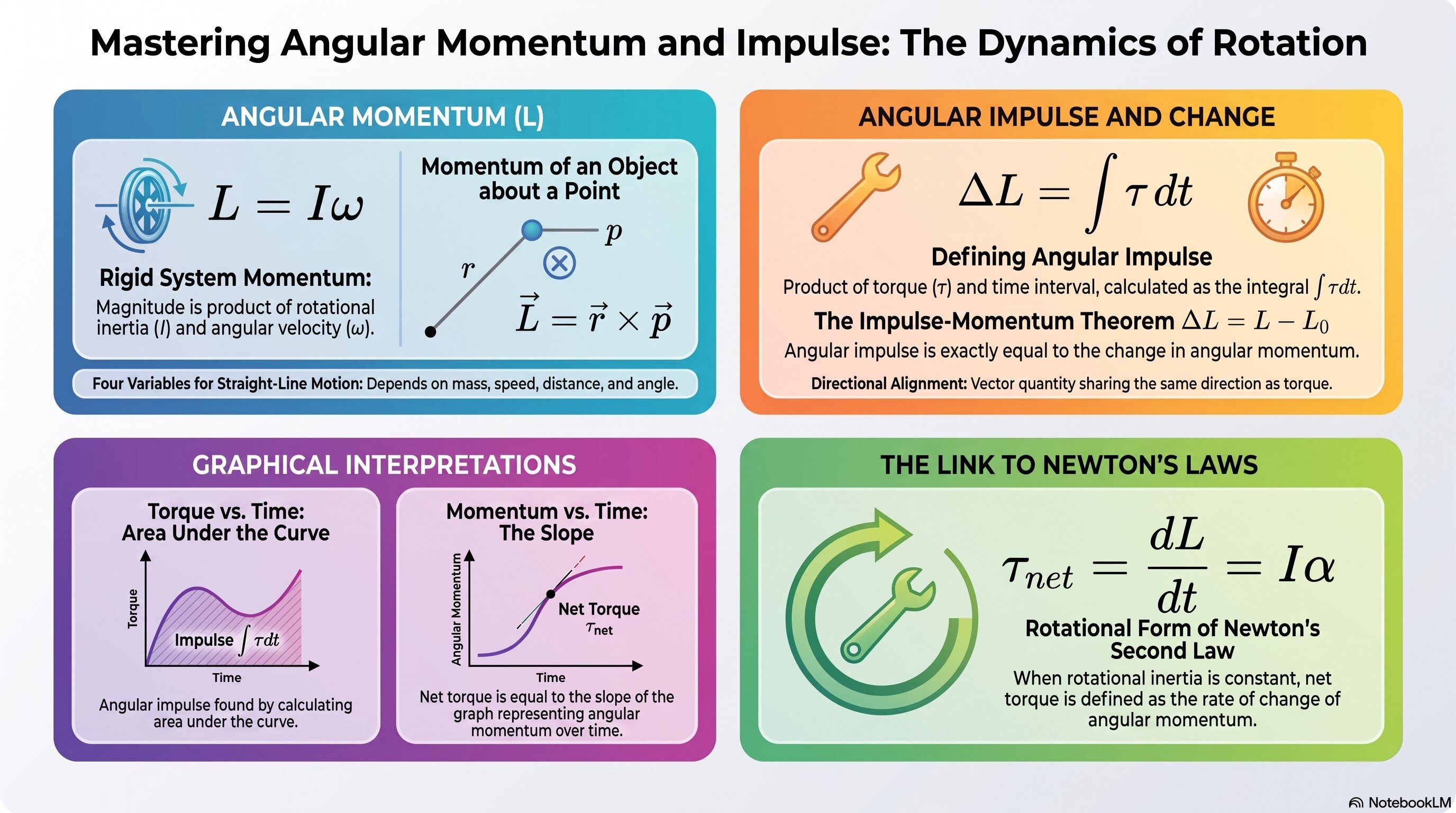
Use this as a quick reference for L = Iω, angular impulse ΔL = τΔt, and both graphical interpretations.
🧭 Plot Summary
In Unit 4 you learned that linear momentum p = mv resists changes in translational motion. This lesson introduces the rotational counterpart: angular momentum L = Iω. A spinning object with large rotational inertia or high angular velocity strongly resists changes to its rotation. This is why gyroscopes stay upright, why a spinning top is hard to knock over, and why figure skaters can control their spin by changing their arm position.
The angular impulse-momentum theorem mirrors the linear version from 4.2 exactly: a net torque acting over time produces a change in angular momentum. J_ang = τΔt = ΔL. And just as F vs. t area gives linear impulse, τ vs. t area gives angular impulse — and the slope of L vs. t gives net torque.
The complete analogy to Unit 4
What you will do in this lesson
- Define angular momentum for a rigid system: L = I*omega (units: kg·m²/s).
- Define angular impulse: J_ang = tau * Dt = DL (angular impulse-momentum theorem).
- Extract angular impulse from the area under a tau vs. t graph.
- Extract net torque from the slope of an L vs. t graph.
- Connect tau_net = dL/dt to tau_net = I*alpha for constant rotational inertia.
- Identify angular momentum as a vector quantity aligned with the rotation axis.
Why it matters
Angular momentum is the key quantity for Lesson 6.4 — conservation of angular momentum. Everything in this lesson is setup for that payoff. The graphical skills (area under τ vs. t, slope of L vs. t) appear on the AP exam and directly transfer from the Unit 4 skills you already know. Master L = Iω and J_ang = ΔL here and 6.4 flows naturally.
✅ Self-Check Before You Roll On
Check off each item as you get there. These are not grades — they are your own signal.