Use this as a quick reference for motion graphs and the kinematic equations.
🧭 Plot Summary
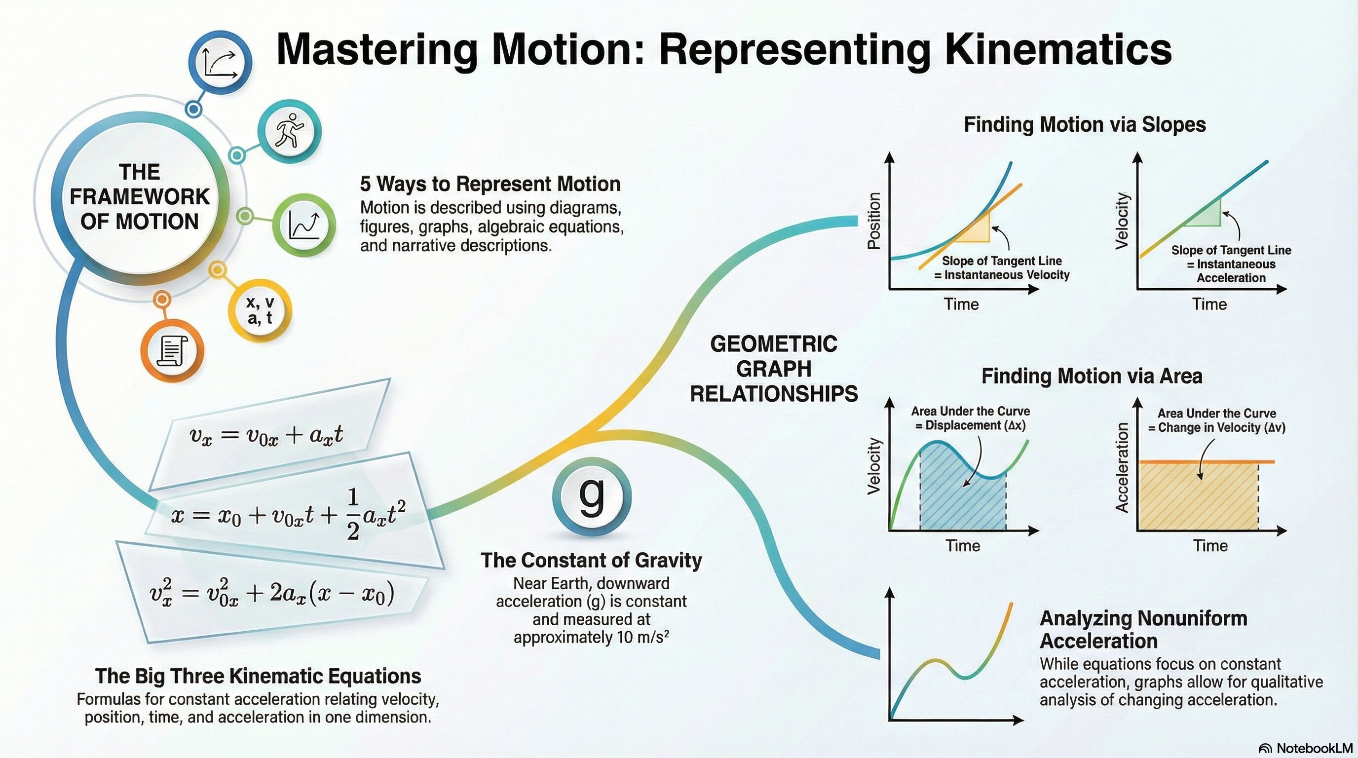
A single motion can be told as a story in many ways: in words, in a data table, with a motion diagram, and — most powerfully — with graphs. In this lesson you'll learn that position-time, velocity-time, and acceleration-time graphs are three views of the same event. The slope of one graph becomes the value of the next, and the area under a graph hands you displacement or change in velocity. Finally, you'll meet the kinematic equations that let you solve constant-acceleration problems with algebra.
What you'll do in this lesson
- Represent one motion in multiple ways: words, tables, motion diagrams, and graphs.
- Connect position-time, velocity-time, and acceleration-time graphs to each other.
- Read slope as a rate of change — slope of x-t is velocity, slope of v-t is acceleration.
- Find displacement and change in velocity from the area under a curve.
- Select and apply the kinematic equations for constant-acceleration motion.
- Treat free fall as constant acceleration with g ≈ 10 m/s².
Why it matters
Graph reading is tested on nearly every AP Physics 1 exam. If you can translate fluidly between a graph, a table, and an equation, you can attack almost any kinematics question — and the same graph-reading skills carry straight into energy, momentum, and circuits later in the course.
✅ Self-Check Before You Roll On
Check off each item as you get there. These aren't grades — they're your own signal.